Image processing is a form of signal processing in which the input “signal” is an image. Typically, the image is considered as a two-dimensional signal, and one or more processes are performed on it. The output of the processes may be an image itself, or it may be a set of characteristics describing the original image.
Deconvolution
Deconvolution is a process that removes or reassigns out-of-focus light in an image, or series of images. In general, two kinds of deconvolution methods are available: optical and computational. Optical methods involve blocking the out-of-focus light before it reaches the detector, as in a confocal microscope. Computational deconvolution methods, typically applied to a wide-field microscope, involve processing a stack of 2-D images by a computer to reduce the out-of-focus contribution in each slice. Computational methods can further be classified as 2-D or 3-D methods. 2-D methods aim to remove the out-of-focus light by comparing a slice with a neighboring slice, while 3-D methods use the point spread function of the system to reassign the out-of-focus light back to the source it originated from.
One area where deconvolution methods are particularly useful is in fluorescence imaging. In this technique, a sample is typically tagged with a fluorophore, meaning that a certain part of the sample gets a substance attached to it which will fluoresce under appropriate conditions. Then, the sample is subjected to a specific light source, defined by the fluorophores present. This light excites the fluorophores to a higher energy state. Then, the fluorophores return to their ground state, thus emitting light of a wavelength separate from that of the excitation light. Deconvolution is suited for this type of imaging for a couple of reasons. For one, the sample emits light which will be imaged in the shape of the point spread function, and therefore must be reassigned. Second, fluorescence imaging usually requires low light levels, meaning that structures may be difficult to see in a raw image, and deconvolution can help to enhance the contrast of these images. For these reasons, as well as many others, deconvolution can prove a helpful tool in fluorescence microscopy.
Object Segmentation

Fig. (a) DIC Image of 293 cells expressing RFP and (b) result of segmentation (centroids and the borders)
Most laboratories studying biological processes use light/fluorescence microscopes to image cells and other biological samples. Quantitative microscopy allows cells migration, differentiation and association to be studied. For these quantitative analysis complex image processing algorithms such as object segmenation should be developed.
Retina samples have been prepared from 3 week and 6 week mice. The eyes were bisected equatorially and the entire retina was removed under the dissecting microscope. Following completion of trypsin digestion, retinal vessels were flattened by four radial cuts and mounted on glass slides. The bright field images (shown above) were acquired with a TiE Nikon inverted microscope. The total number of endothelial cells and pericytes were detected and counted using a marker based watershed segmentation algorithm. The location of foreground markers (cells) is detected using the center and surround method and the background markers were computed by watershed detection on the resulted binary mask. Then the gradient of the images(d) is calculated and modified to enforce local minima in foreground and background objects(e). The watershed transform of the modified gradient image is computed as the binary mask containing the objects(f).
Retinal Vasculature Feature Extraction
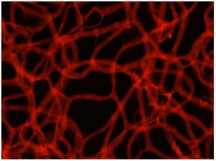
After the mice had reached either 3 or 6 weeks of age, they were sacrificed and the retinas were extracted. The retinal wholemounts obtained were stained with anti-PECAM-1 antibody to allow for imaging. They were incubated with rabbit anti-PECAM-1 at 4°C overnight. The retinas were washed with PBS, and incubated with Alexa 594 goat-anti-rabbit for 2 hours at room temperature. This staining allows for fluorescence imaging of the retinal vasculature using a green excitation and red emission filter pair. Finally, the retinas were washed four times with PBS at 30 minutes each, and mounted on a slide using a mixture of PBS and glycerol.
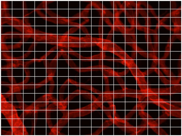
The fractal dimension of the vasculature was determined using the box counting method. In this method, the original image is divided up into smaller regions, and the number of these smaller regions containing part of the vasculature is counted. This process is repeated for many sizes of small regions, and the relationship between the size of the regions and the number required to cover the vasculature was determined. This relationship is then fit to a power law using least squares regression, and the resulting exponent is recorded as the fractal dimension.
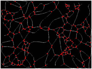
The location of points of overlap and branching between vessels was determined by first reducing all vessels to a pixel width of 1, using morphological thinning. Then, the branch points of the thinned vasculature are found by looking at each individual pixel’s immediate neighborhood for areas of background and vasculature. The vessel caliber is determined as the average width of a vessel throughout the vasculature. To extract this feature, the vasculature is first thinned and the location of branch points determined (see points of overlap). Then, in areas of the image which are part of the thinned vasculature, but not near a branch point, a small sub-region is selected. This sub-region is rotated by 90° to obtain a line normal to the vessel in the same sub-region. The sum of the overlap of this line with the original vasculature in the same sub-region is recorded as the vessel width at the current point. This process is then repeated for all pixels which meet the above criteria, and the average of these values is the vessel caliber.
Reconstruction and 3D rendering of the cryoimagers results and comparison
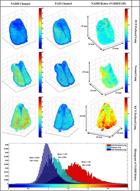
Representative 3D reconstructions of lungs from three groups (normoxic, normoxic + KCN, and Normoxic + PCP). Images were acquired form the cryoimager with the resolution of 40u in x, y and z directions and processed in matlab. From left to right, images shown are NADH, FAD, and mitochondrial redox ratio (RR). The bottom panel shows the histogram distribution of Redox ratio for the three lungs shown above.